
Aquarium object detection #2 - YOLOv5 baseline
Table of contents
This article is part #2 of a series about aquarium object detection
1. Default YOLOv5 training
We will start our object detection journey by developing a baseline model. This model will be our point of reference for further experiments. The aquarium dataset on Roboflow offers access to the already trained YOLOv5 model. The model tab reports 74% mAP@0.5 on a validation set and 73% mAP@0.5 on a test set.
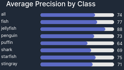
Validation set metrics
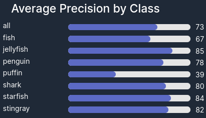
Test set metrics
We’ll try to recreate these results as our baseline.
YOLOv5 is a single-stage object detector released in 2020, which at the time claimed to offer state-of-the-art object detection. Its easy-to-use framework made it a popular choice, especially among practitioners. While YOLOv5 is no longer state-of-the-art, it remains a reasonable out-of-the-box option for establishing a baseline model.
For our training and evaluation notebooks we will use packaged version of YOLOv5, which is a Python wrapper for ultralytics/YOLOv5 scripts. The package is available through pip and offers some additional useful features including integration with HuggingFace Hub.
1.1 Training code
Training notebook is available on GitHub and in Google Colab:
![]()
Dataset download
Before the training, we first have to download data. We will again use Roboflow, but this time we will download data already in YOLOv5 format.
%env ROBOFLOW_API_KEY=#########
!curl -L "https://universe.roboflow.com/ds/aXGylruXWt?key=$ROBOFLOW_API_KEY" > roboflow.zip
!unzip -o -q roboflow.zip -d data && rm roboflow.zip
Unfortunately downloaded dataset misses information about the dataset root directory in the data.yaml file.
We have to insert this path ourselves in the first line of the file.
!sed -i "1i path: /content/data" data/data.yaml
There is one more thing we have to do before running training. During exploratory data analysis, we found out that one of the images is mislabeled. Let’s correct the annotations for this image. We will simply replace all category ids with 1 (jellyfish) as the image contains only jellyfish objects.
%env mislabeled_file=data/train/labels/IMG_8590_MOV-3_jpg.rf.e215fd21f9f69e42089d252c40cc2608.txt
!awk '{print "1", $2, $3, $4, $5}' $mislabeled_file > tmp.txt && mv tmp.txt $mislabeled_file
Training
Running training requires just a few lines of code.
from yolov5 import train

train.run(imgsz=640,
          epochs=300,
          data='data/data.yaml',
          weights='yolov5s.pt',
          logger='TensorBoard',
          cache='ram');
With this code we will train a “small” model starting from COCO-pretrained weights (yolov5s.pt), using default hyperparameters. The image size is set to 640, which is also a default. Training will run for 300 epochs. TensorBoard was selected as a logger, so we can run it in a notebook to monitor the progress of the training.
%load_ext tensorboard
%tensorboard --logdir runs/train
We also opted to cache images in memory with the cache='ram' option as it drastically shortens training time. Training of a small model for 100 epochs takes over 3 hours without caching and around 18 minutes with memory caching – that is 10x faster! (training on NVIDIA V100 GPU)
1.2 Training results
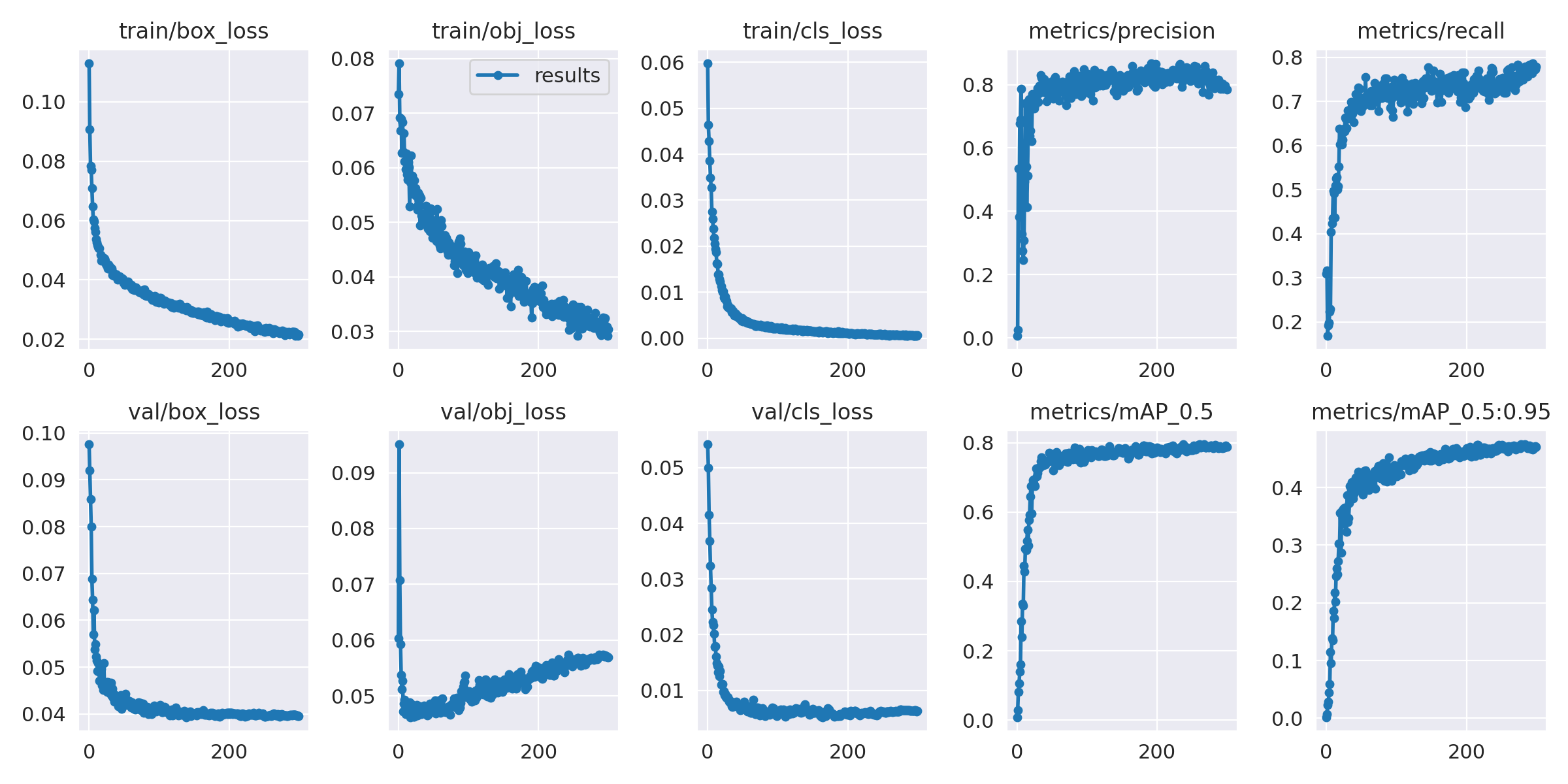
Results of our first training are available in runs/train/exp directory. Let’s compare our “small” model training charts with training charts for the Roboflow model.
Our model
Roboflow model
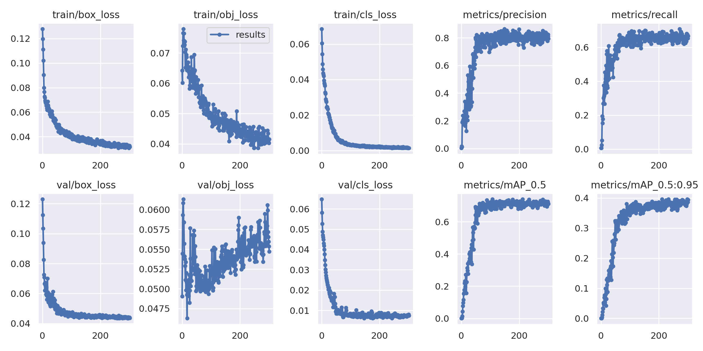
We can see that both plots are very similar. Let’s also compare the validation set mAP@0.5 metrics reported at the end of the training to get a better understanding of the results.
| Roboflow | Our model | |
|---|---|---|
| All | 0.74 | 0.795 |
| Fish | 0.77 | 0.838 |
| Jellyfish | 0.88 | 0.956 |
| Penguin | 0.73 | 0.719 |
| Puffin | 0.64 | 0.616 |
| Shark | 0.69 | 0.8 |
| Starfish | 0.75 | 0.819 |
| Stingray | 0.71 | 0.815 |
We managed to recreate baseline results from the Roboflow model and obtained even better results out-of-the-box, with default training settings:
- The overall mAP improved by over five percentage points
- We also see an improvement in the metrics for each of the classes except for the puffin
- The model seems to be undertrained and it looks like there is room for improvement with longer training
I would attribute such significant improvement to one of the two things. Roboflow model could be an even smaller, less capable, YOLOv5n (“nano”) model – unfortunately, I haven’t found information about model size on the Roboflow page. The second option is that both models are “small” models and improvements come from enhanced training routine, better data augmentation, modified default hyperparameters, or other changes introduced with new YOLOv5 releases.
We used validation set metrics as a first point of reference for model performance. This makes sense since we didn’t use a validation set to tune the hyperparameters. Later on, we will conduct more detailed evaluations with the test set.
2. Training improvement
2.1 Limiting objectness loss gain
There is one more clear conclusion coming from the above training results – validation objectness loss is overfitting from early epochs, while other loss components are still decreasing. YOLOv5 loss function consists of three weighted components:
- Location (box) loss
- Objectness loss
- Classes loss
To eliminate observed overfitting we can try to decrease the weight (gain) associated with the objectness component. In YOLOv5 objectness loss gain is defined as obj hyperparameter. Let’s first update our training script to allow the modification of hyperparameters.
YOLOv5 uses .yaml files to store hyperparameter config. Default hyperparameters are defined in hyp.scratch-low.yaml file. We could just manually download and modify this file, however, let’s develop a solution that doesn’t require any manual file manipulation. By following this approach, we can eliminate the need for manual file uploads in Google Colab and use Python code to modify the default config.
import yaml
import torch

# Default hyperparameters config
hyp_file = 'hyp.scratch-low.yaml'
hyp_url = f'https://raw.githubusercontent.com/ultralytics/yolov5/master/data/hyps/{hyp_file}'

# Get default hyperparameters config
torch.hub.download_url_to_file(hyp_url, hyp_file)

# Load YAML into dict
with open(hyp_file, errors='ignore') as f:
    hyps = yaml.safe_load(f)

# MODIFY HYPERPARAMETERS
hyps['obj'] = 0.3

# Dump dict into YAML file
with open(hyp_file, 'w') as f:
  yaml.dump(hyps, f, sort_keys=False)
Default hyperparameters are loaded into the hyps dictionary and can be modified there. Dictionary is later dumped back to the .yaml file. If no changes are applied, then we just train with the default config from hyp.scratch-low.yaml.
To run the training with modified hyperparameters we just need to pass the hyp argument to train.run().
train.run(imgsz=640,
          epochs=300,
          data='data/data.yaml',
          weights='yolov5s.pt',
          logger='TensorBoard',
          cache='ram',
          hyp=hyp_file)
2.2 Improved training results
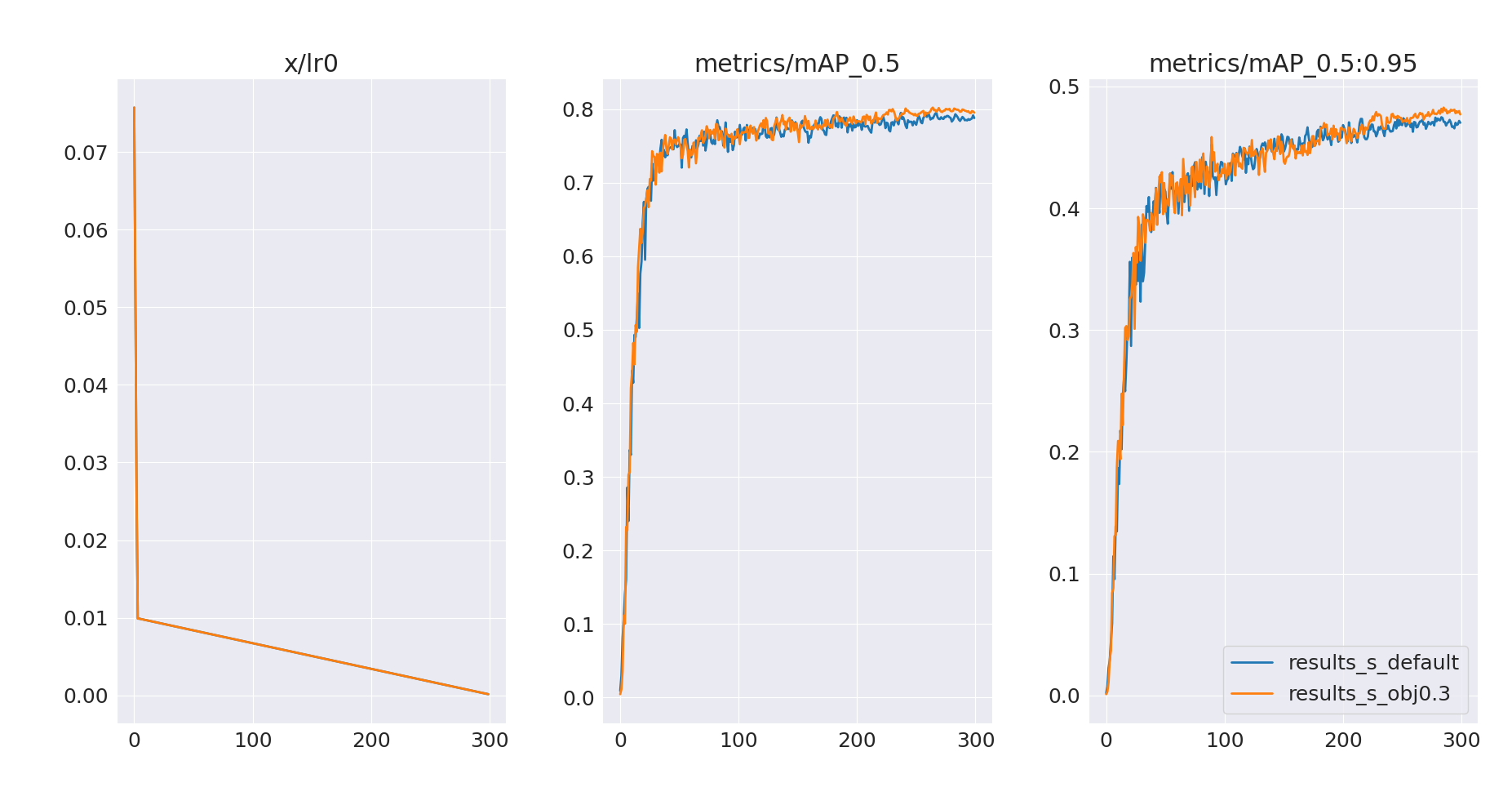
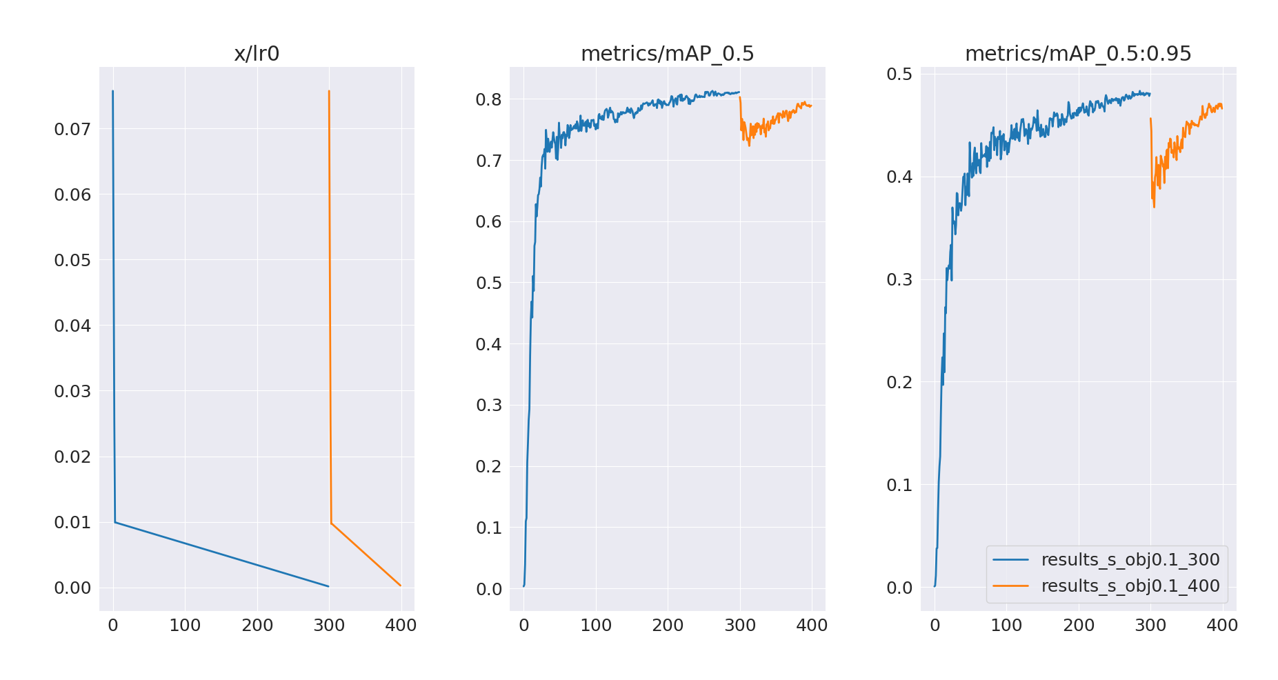
Let’s now train with an arbitrarily selected objectness gain value of 0.3 (default value is 1.0). The result of this run is presented below, with the default run (results_s_default) as a reference.
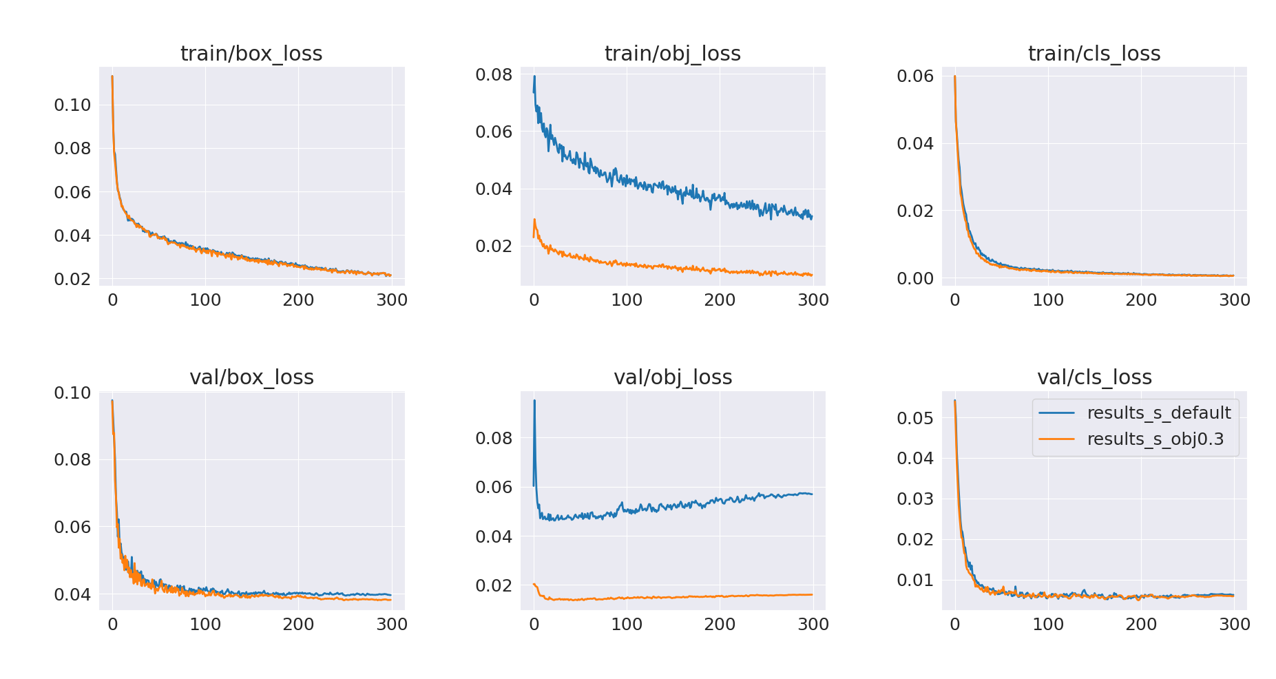
It looks like objectness loss is still overfitting. Let’s run another training with an even smaller gain of 0.1
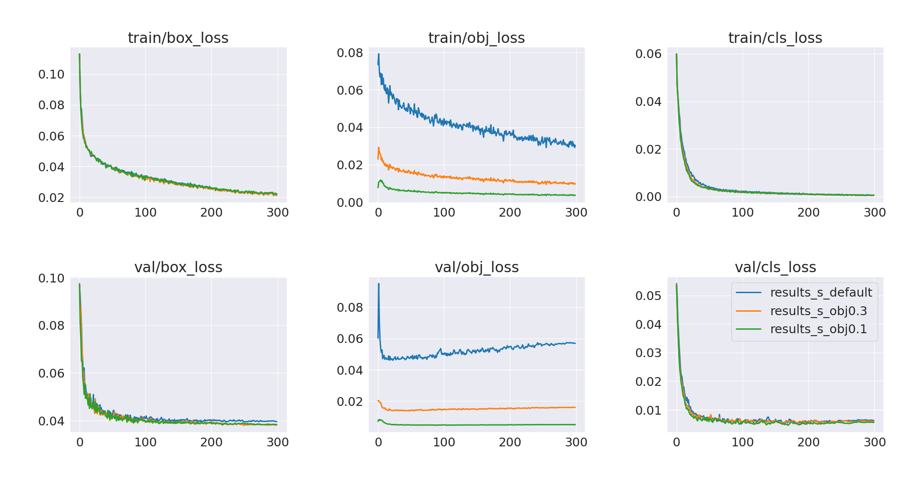
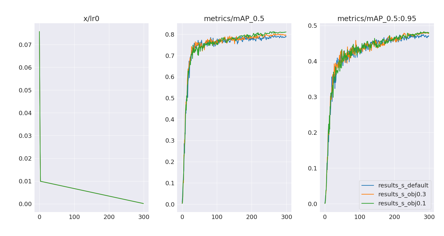
This experiment looks more promising – we’ve mitigated the overfitting issue, and validation mAP@0.5 after 300 epochs has improved.
However, it also looks like the models are still undertrained and could benefit from longer training:
- Validation loss (box/cls) is still decreasing
- Validation mAP keeps increasing
2.3 Longer training
Let’s train the two models (default and one with obj=0.1) for another 100 epochs and see if they can improve further. To continue training we can just supply last.pt or best.pt weights from previous trainings to a new train.run() call – new training will start from our already trained weights instead of COCO-pretrained weights.
train.run(imgsz=640,
          epochs=100,
          data='data/data.yaml',
          weights='best.pt',
          logger='TensorBoard',
          cache='ram',
          hyp=hyp_file)
There is however one more issue. By default YOLOv5 applies warmup epochs and warmup bias in its learning rate scheduler.
# hyp.scratch-low.yaml
...
warmup_epochs: 3.0  # warmup epochs (fractions ok)
warmup_momentum: 0.8  # warmup initial momentum
warmup_bias_lr: 0.1  # warmup initial bias lr
...
If we continue training with these hyperparameters we will get suboptimal results. The initial learning rate is very high, and therefore training is very unstable – in a sense, the model forgot part of the previous training.
Our problem comes from the warmup_bias_lr: 0.1 hyperparameter, which sets initial learning rate to 0.1. We can just change it to 0.0 in our training script in the same way as with obj hyperparameter before.
hyps['warmup_bias_lr'] = 0.0
Longer training without warmup bias
Let’s now run longer trainings without warmup bias. We will also lower the learning rate to lr=0.001 (from default lr=0.01) to avoid problems with stability.
hyps['warmup_bias_lr'] = 0.0
hyps['lr0'] = 0.001
Results of these trainings are presented below.
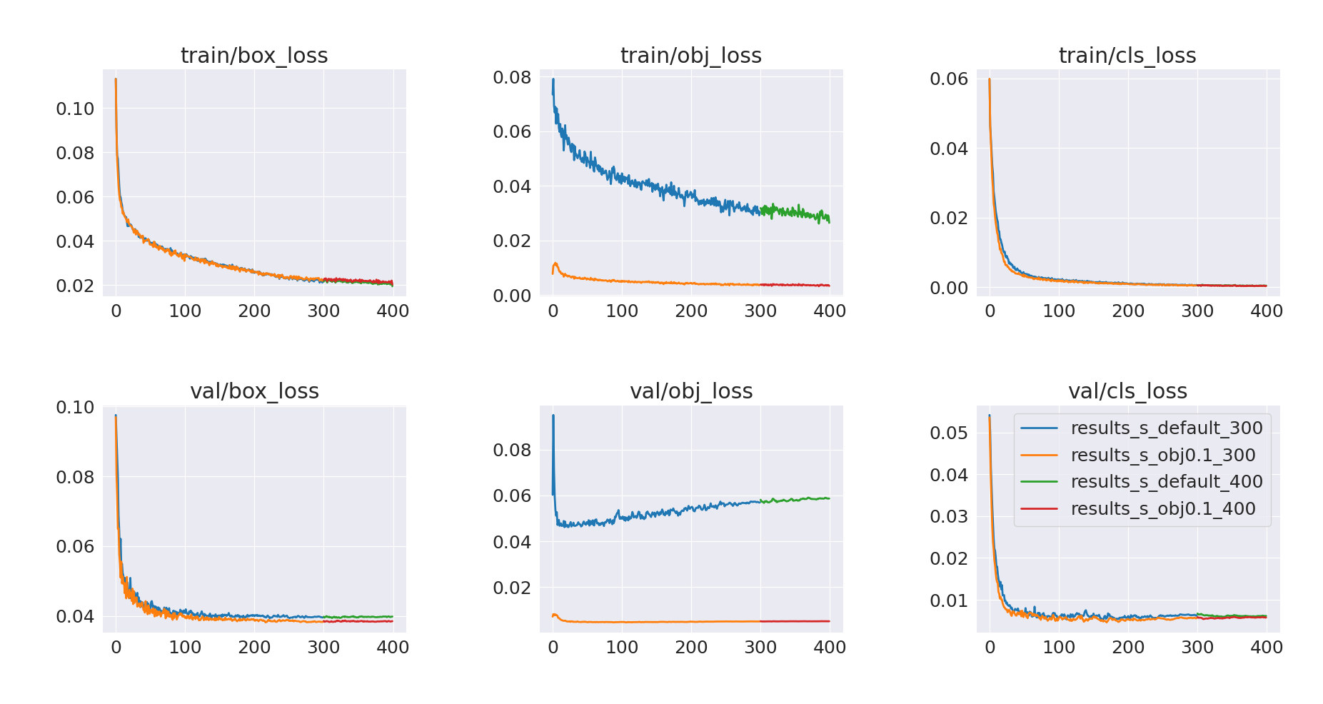
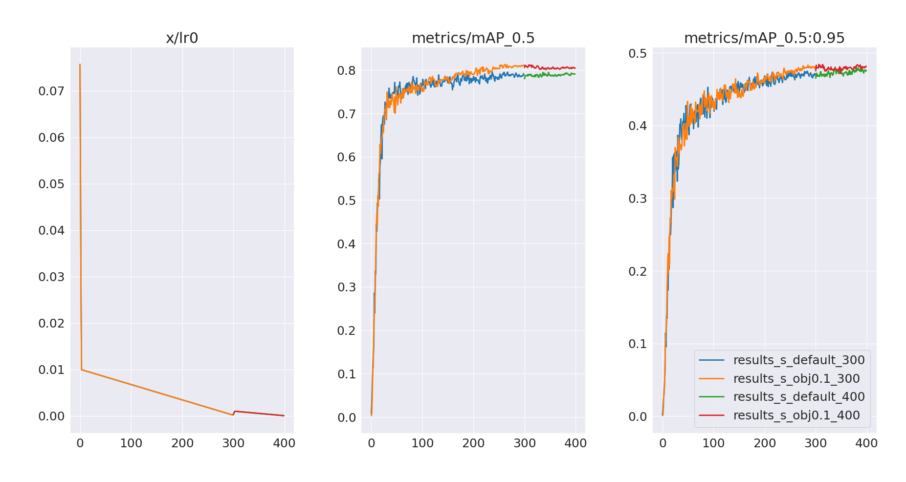
We can see that mAP@0.5 for both models hasn’t really improved, and neither did mAP@0.5:0.95 for obj=0.1 model. In contrast, the default model saw a slight improvement in mAP@0.5:0.95, with a further increasing trend. Let’s also compare per-class mAP values on a validation set for best.pt models after 300 and 400 epochs.
| Roboflow | Our default model (300 epochs) | Our obj=0.1 model (300 epochs) | Our default model (400 epochs) | Our obj=0.1 model (400 epochs) | |
|---|---|---|---|---|---|
| All | 0.74 | 0.795 | 0.81 | 0.788 | 0.812 |
| Fish | 0.77 | 0.838 | 0.842 | 0.843 | 0.838 |
| Jellyfish | 0.88 | 0.956 | 0.952 | 0.934 | 0.954 |
| Penguin | 0.73 | 0.719 | 0.753 | 0.724 | 0.743 |
| Puffin | 0.64 | 0.616 | 0.637 | 0.597 | 0.651 |
| Shark | 0.69 | 0.8 | 0.798 | 0.778 | 0.808 |
| Starfish | 0.75 | 0.819 | 0.868 | 0.806 | 0.861 |
| Stingray | 0.71 | 0.815 | 0.822 | 0.831 | 0.825 |
It seems that obj=0.1 models generally perform better and that longer training brought only little if any improvement. We could of course try to train these models for even longer or experiment with different hyperparameters. But let’s finish the training here and move to the model evaluation, where we will compare both models on an unbiased test set to get a better understanding of their performance and the ability to generalize to unseen data.
3. Model evaluation
Before we start evaluation, it is important to note that our test set is relatively small. Comparison of test-set metrics might not reflect the true performance of the models on the unseen data. This is particularly noticeable for less numerous classes, where changes in metrics might be abrupt – for example, there are only 11 starfish objects in our test set.
YOLOv5 has an evaluation script that calculates the most important metrics out-of-the-box. A simple evaluation notebook can be found on GitHub and in Google Colab:
![]() .
We download the Roboflow dataset with the same code as in the training notebook, and then we can just run the evaluation, selecting data split with the
.
We download the Roboflow dataset with the same code as in the training notebook, and then we can just run the evaluation, selecting data split with the task keyword.
from yolov5 import val

weights = 'best.pt'
# weights = 'akbojda/yolov5s-aquarium'

val.run(imgsz=640,
        data='data/data.yaml',
        weights=weights,
        task='test')
Of course, we also have to provide the weights of the model that we want to evaluate. One way is to just pass the path to the local .pt file as we did before. The other interesting option is to upload the model to the HuggingFace Model Hub. Packaged YOLOv5 has full HuggingFace Hub integration – we can just use the model name and it will be downloaded under the hood. For example, weights = 'akbojda/yolov5s-aquarium' will use this model that I uploaded to the 🤗 Hub.
3.1 Comparison of mean average precisions
Let’s first take a look at the values of mAP@0.5 and mAP@0.5:0.95 calculated on the test dataset, for different models.
| Roboflow | Our default model (300 epochs) | Our obj=0.1 model (300 epochs) | Our default model (400 epochs) | Our obj=0.1 model (400 epochs) | |
|---|---|---|---|---|---|
| All | 0.73 | 0.813 | 0.854 | 0.808 | 0.847 |
| Fish | 0.67 | 0.783 | 0.809 | 0.766 | 0.812 |
| Jellyfish | 0.85 | 0.892 | 0.909 | 0.865 | 0.905 |
| Penguin | 0.78 | 0.825 | 0.828 | 0.806 | 0.815 |
| Puffin | 0.39 | 0.561 | 0.666 | 0.54 | 0.642 |
| Shark | 0.8 | 0.832 | 0.817 | 0.843 | 0.81 |
| Starfish | 0.84 | 0.952 | 0.971 | 0.956 | 0.976 |
| Stingray | 0.82 | 0.847 | 0.98 | 0.882 | 0.971 |
| Roboflow | Our default model (300 epochs) | Our obj=0.1 model (300 epochs) | Our default model (400 epochs) | Our obj=0.1 model (400 epochs) | |
|---|---|---|---|---|---|
| All | - | 0.497 | 0.519 | 0.492 | 0.513 |
| Fish | - | 0.469 | 0.48 | 0.461 | 0.482 |
| Jellyfish | - | 0.584 | 0.605 | 0.582 | 0.603 |
| Penguin | - | 0.371 | 0.362 | 0.364 | 0.36 |
| Puffin | - | 0.277 | 0.324 | 0.241 | 0.31 |
| Shark | - | 0.537 | 0.544 | 0.549 | 0.545 |
| Starfish | - | 0.604 | 0.621 | 0.627 | 0.613 |
| Stingray | - | 0.635 | 0.698 | 0.618 | 0.678 |
Clearly, models trained with limited objectness gain (obj=0.1) perform better compared to the default training configuration. It also seems that extended training hasn’t improved the overall performance. In conclusion: the obj=0.1 model trained for 300 epochs looks to be the best choice.
3.2 Precision-Recall and F1-score curves
Let’s take a closer look at other metrics of this model, starting with the evaluation summary generated with the val.run call. mAP values are identical as in the comparison tables above. Precision and recall values are reported at the maximum F1-score confidence threshold.
| Images | Labels | Precision | Recall | mAP@.5 | mAP@.5:.95 | |
|---|---|---|---|---|---|---|
| All | 63 | 584 | 0.897 | 0.756 | 0.854 | 0.519 |
| Fish | 63 | 249 | 0.808 | 0.735 | 0.809 | 0.480 |
| Jellyfish | 63 | 154 | 0.885 | 0.877 | 0.909 | 0.605 |
| Penguin | 63 | 82 | 0.834 | 0.793 | 0.828 | 0.362 |
| Puffin | 63 | 35 | 0.855 | 0.571 | 0.666 | 0.324 |
| Shark | 63 | 38 | 0.963 | 0.694 | 0.817 | 0.544 |
| Starfish | 63 | 11 | 0.935 | 0.909 | 0.971 | 0.621 |
| Stingray | 63 | 15 | 1.000 | 0.714 | 0.980 | 0.698 |
The validation script also plots Precision-Recall, Precision-Confidence, Recall-Confidence, and F1-Confidence curves.
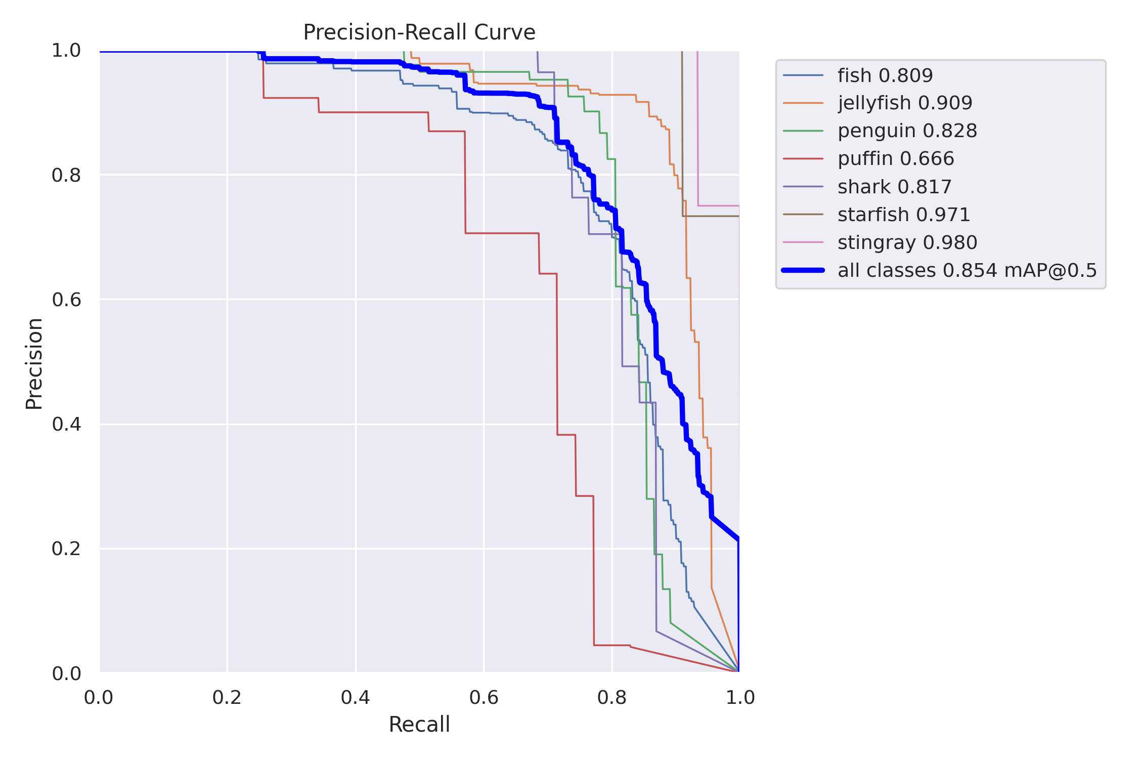
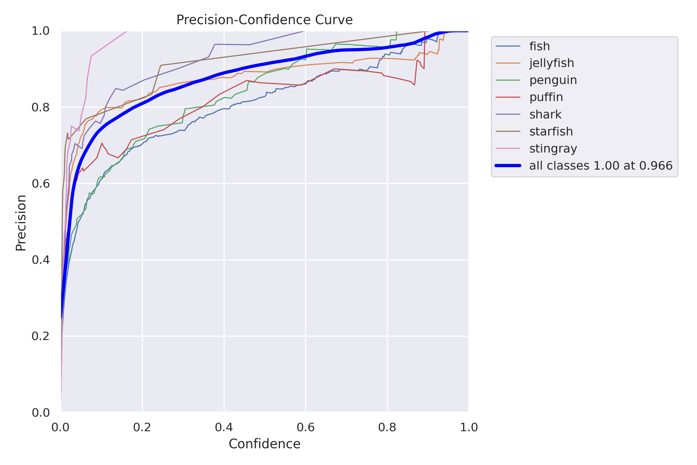
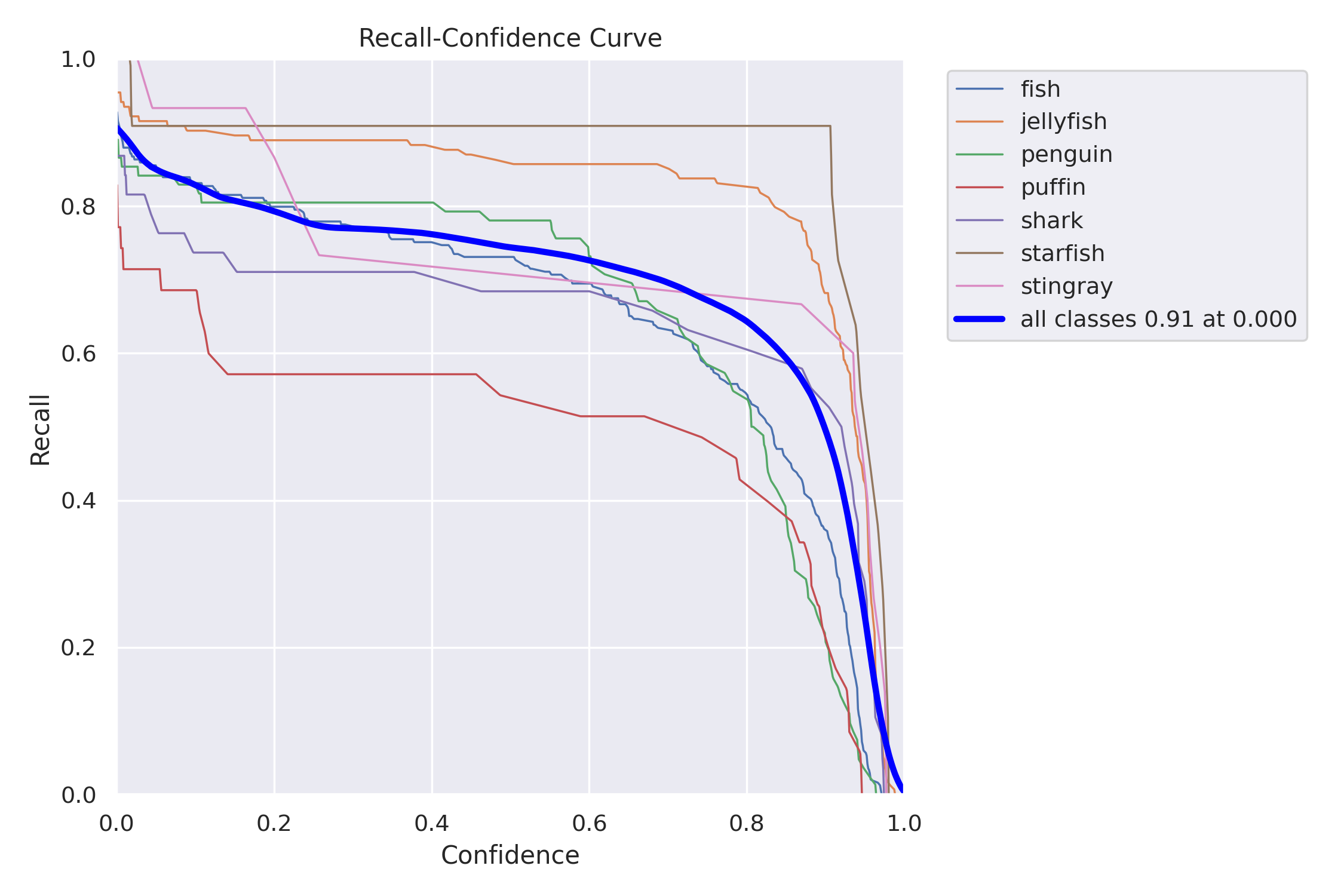
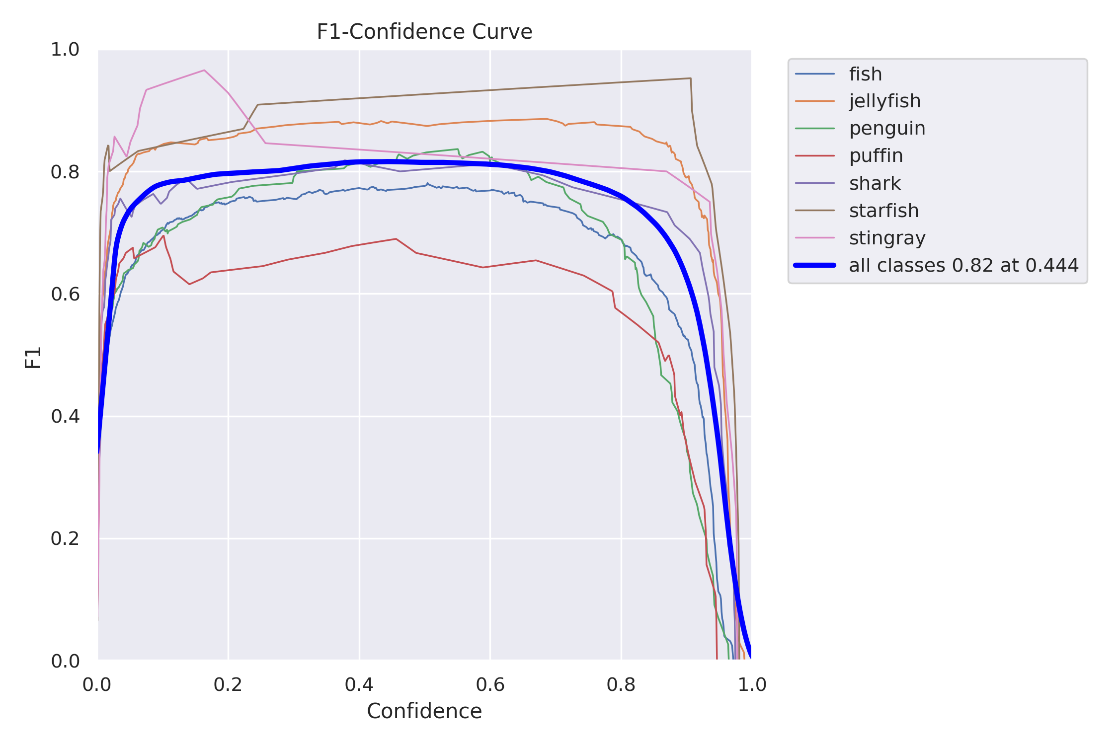
In object detection we always face a trade-off between precision and recall:
- When we cannot afford to miss any detection, we look for high recall
- When we cannot afford to have any incorrect detection we look for high precision
We can use the above charts to select a confidence threshold that gives us the desired trade-off between precision and recall. If we don’t have a strong preference for one of the metrics, we can use the F1-score, which is the harmonic mean of precision and recall. On the F1-Confidence curve, we can see that the highest F1 score (combined for all classes) has a value of 0.82, and is obtained at a 0.444 confidence threshold. We can also find this threshold in the Precision-Confidence and Recall-Confidence charts and confirm values reported in the evaluation summary table – precision=0.897 and recall=0.756.
It is also worth noting that we obtain very similar F1 scores for confidence thresholds in a range between 0.15 and 0.65 – these values seem to be good threshold candidates if we want to optimize recall or precision respectively.
Let’s compare precision and recall values at these three different confidence thresholds.
| Confidence threshold | Precision | Recall |
|---|---|---|
| 0.15 | 0.78 | 0.805 |
| 0.444 | 0.897 | 0.756 |
| 0.65 | 0.945 | 0.71 |
We can observe the precision-recall trade-off that comes with these different thresholds. For our detection task threshold of 0.444 seems to be a good choice as we don’t have a strong preference for either precision or recall, and want balanced performance.
3.3 Confusion matrix
Let’s also take a look at the confusion matrix.
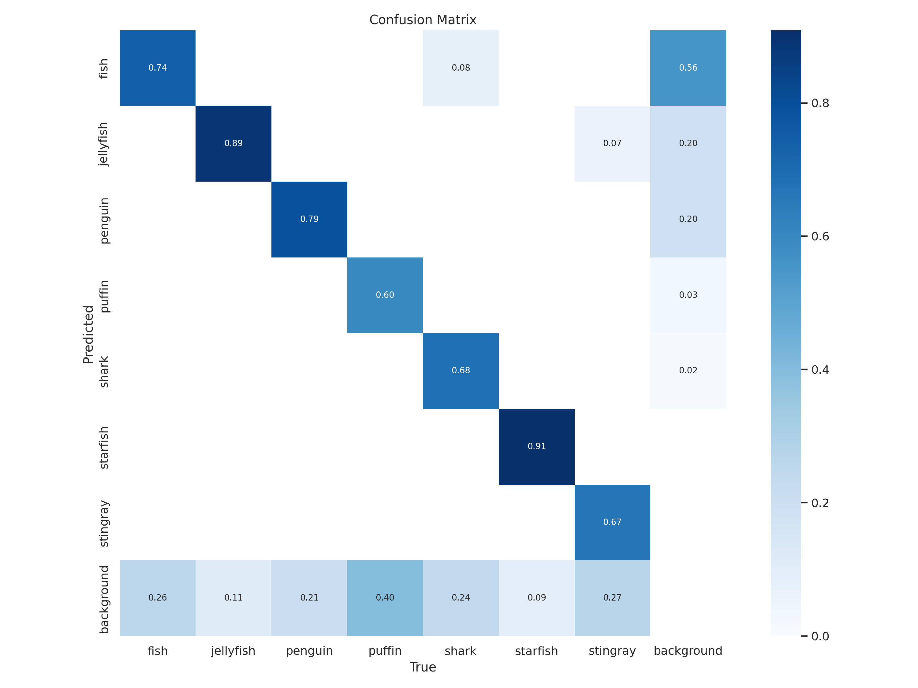
The confusion matrix won’t be very useful for analyzing false negatives and false positives – we already did it by looking at precision and recall curves (overall and per-class). But we can use this matrix to verify some conclusions we came up with during exploratory data analysis (part 1 of the series) and make some new observations:
| EDA observation | Confusion matrix observation |
|---|---|
| "Fish, sharks, and stingrays are relatively similar animals, which might be misidentified, especially in adverse conditions" | Partially true – we can see that sharks are sometimes detected as fish |
| "Penguins and puffins are relatively similar animals, which might be misidentified" | False – we can see that these classes aren't misidentified |
| "There are two classes, which are quite distinctive and not similar to the others: jellyfish and starfish" | 50/50 – jellyfish and starfish aren't actually misidentified, but stingrays are identified as jellyfish in some situations |
3.4 Predictions vs ground-truth annotations
The last thing we will do as part of the model validation will be to look at the predictions for specific images and compare them to ground-truth annotations. The validation script already outputs some detection results in the form of mosaics – ground truth annotations are on the left and our model predictions are on the right.
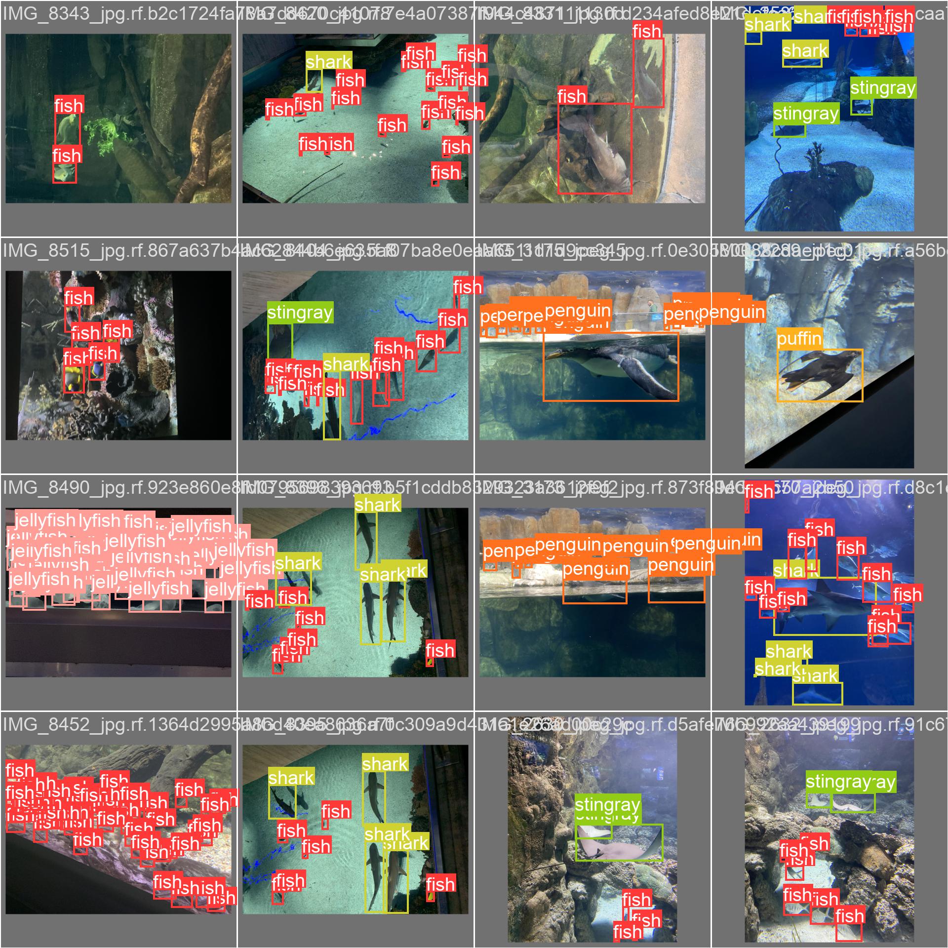
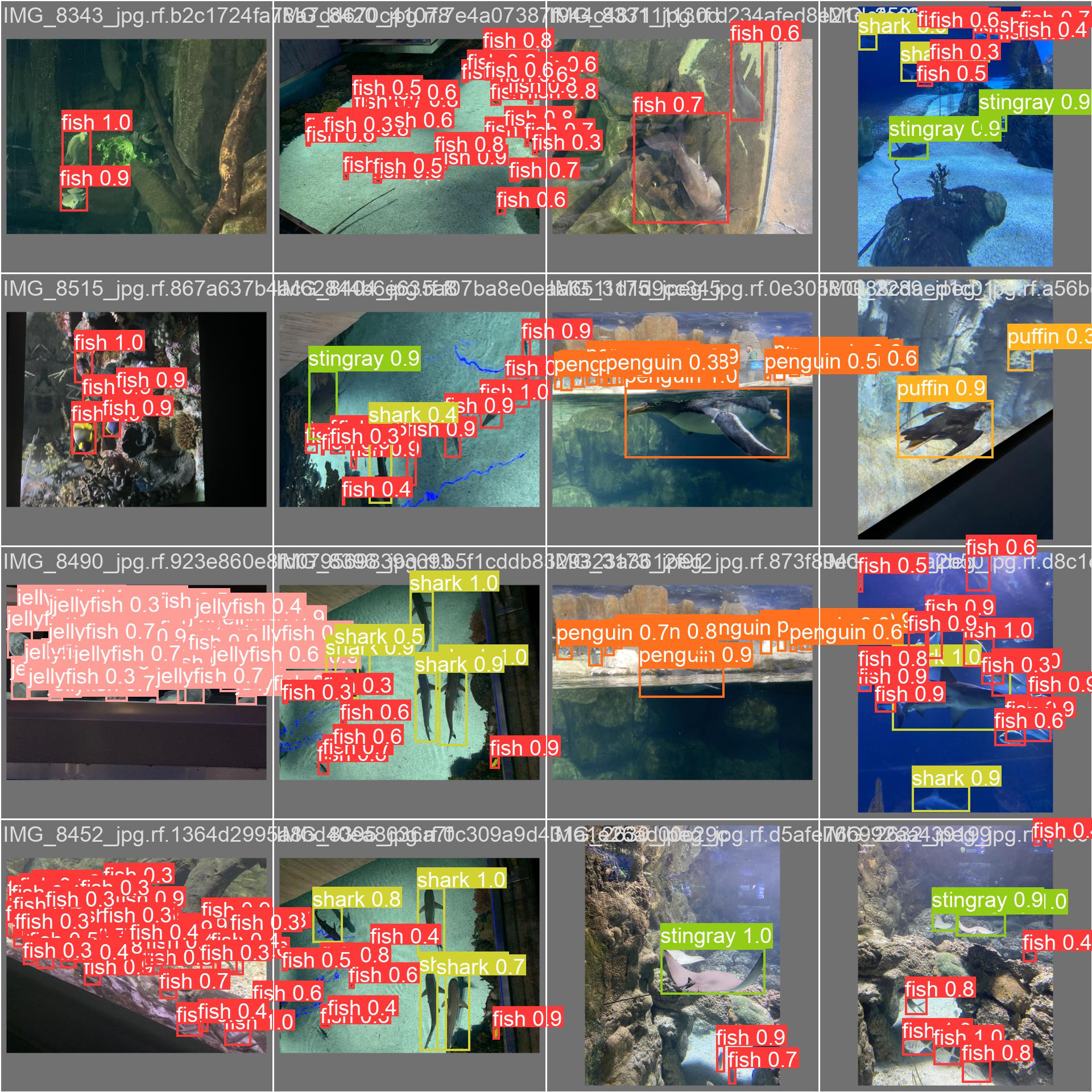
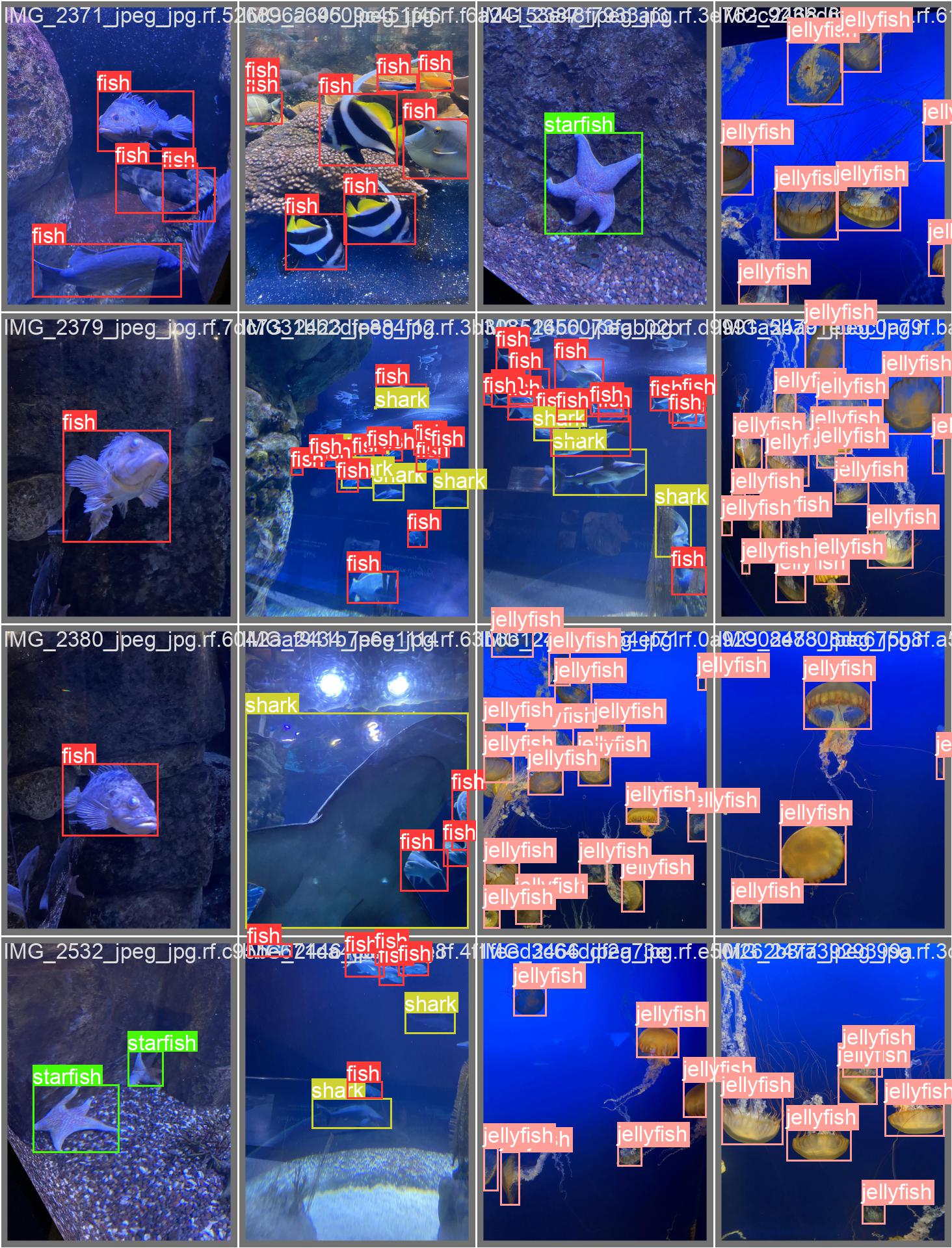
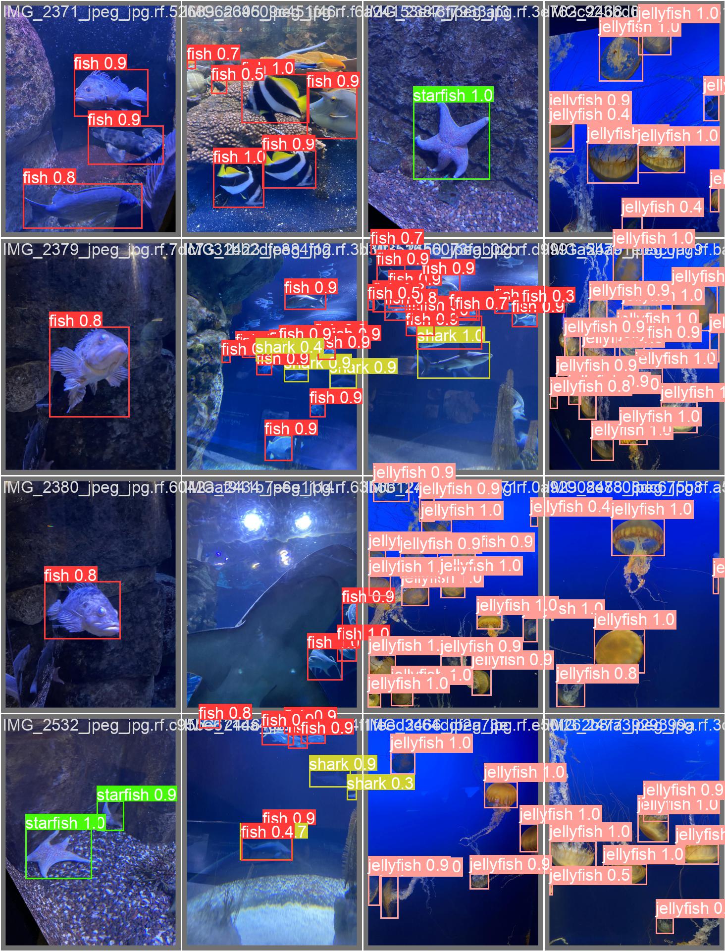
However, these mosaics contain only part of the test set. Also, images containing multiple objects are unreadable. Let’s instead download model predictions in COCO-json format – we can do it with the save_json=True argument passed to validation run.
val.run(imgsz=640,
        data='data/data.yaml',
        weights=weights,
        task='test',
        save_json=True)
Unfortunately, exported file contains only a list of annotations, and misses information about images or metadata. Moreover, image_id field in annotations contains the filename instead of the image id as defined in COCO data format.
To fix this, I first copied missing information from the ground-truth annotation file (and removed the “creatures” supercategory from categories list). Then, I used the following script to rewrite the image_id field in annotations.
import json

def get_image_id(name, images):
    for image in images:
        if image['file_name'] == f'{name}.jpg':
            return image['id']

    raise ValueError(name)

if __name__ == '__main__':
    with open('predictions_fixed.json', 'r') as in_f:
        data = json.load(in_f)

    for ann in data['annotations']:
        ann['image_id'] = get_image_id(ann['image_id'], data['images'])

    with open('predictions_fixed.json', 'w') as out_f:
        json.dump(data, out_f)
The resulting file can be seen here.
Predictions analysis with FiftyOne
To compare ground-truth annotations with model predictions we will use FiftyOne – the library that we already used during exploratory analysis. Notebook with this part of the evaluation can be found on GitHub and in Google Colab:
![]() .
Loading ground-truth annotations and predictions is straightforward.
.
Loading ground-truth annotations and predictions is straightforward.
import fiftyone as fo

dataset = fo.Dataset.from_dir(
    name='Aquarium Combined',
    dataset_type=fo.types.COCODetectionDataset,
    data_path='test',
    labels_path='test/_annotations.coco.json',
    label_field='ground_truth',
)

pred_dataset = fo.Dataset.from_dir(
    dataset_type=fo.types.COCODetectionDataset,
    data_path='test',
    labels_path='predictions_fixed.json',
    label_field='model',
)

dataset.merge_samples(pred_dataset)

session = fo.launch_app(dataset)
Now, we can easily use FiftyOne to i.e. compare ground-truth annotations with model predictions, at different confidence levels.
4. Summary
In this article, we managed to establish a baseline model, tested some straightforward improvement ideas, and evaluated trained models. There are of course other aspects we could explore, including running experiments with larger (m/l/x) models or doing hyperparameter optimization. But we will end here as we’ve achieved our two main goals of understanding the YOLOv5 framework and establishing a baseline model.